Texture analysis of 2D data in GSAS-II

· A video version of this tutorial is available at https://anl.box.com/v/Textureanalysisof2DdatainGSAS-

· Exercise files are found here

Introduction

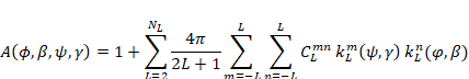
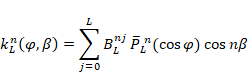
Texture analysis using GSAS-II employs spherical harmonics modeling, as described by Bunge, "Texture Analysis in Materials Science" (1982), and implemented by Von Dreele, J. Appl. Cryst., 30, 517-525 (1997) in GSAS. The even part of the orientation distribution function (ODF) via the general axis equation

is used to give the intensity corrections due to texture. The two harmonic terms, and , take on values according to the sample and crystal symmetries, respectively, and thus the two inner summations are over only the resulting unique, nonzero harmonic terms. These unique terms are automatically selected by GSAS-II according to the space group symmetry and the user chosen sample symmetry. The available sample symmetries are cylindrical, 2/m, mmm and no symmetry. The choice of sample symmetry profoundly affects the selection of harmonic coefficients. For example, in the case of cylindrical sample symmetry (fiber texture) only terms are nonzero so the rest are excluded from the summations and the set of coefficients is sufficient to describe the effect on the diffraction pattern due to texture. The crystal harmonic factor, , is defined for each reflection, h, via polar and azimuthal coordinates (f, b) of a unit vector coincident with h relative to the reciprocal lattice. For most crystal symmetries, f is the angle between h and the n-th order major rotation axis of the space group (usually the c-axis) and b is the angle between the projections of h and any secondary axis (usually the a-axis) onto the normal plane. In a similar way the sample harmonic factor, , is defined according to polar and azimuthal coordinates (y, g) of a unit vector coincident with the diffraction vector relative to a coordinate system attached to the external form of the sample. For example, in the case of a rolled steel plate having mmm symmetry, the polar angle, y, is frequently measured from the normal direction (ND, parallel to K_s) and g is then measured from the rolling direction (RD, parallel to I_s) in the TD (transverse direction, parallel to J_s) - RD plane. Thus, the general axis equation becomes

In a diffraction experiment the crystal reflection coordinates (f, b) are determined by the choice of reflection index (hkl) while the sample coordinates (y, g) are determined by the sample orientation on the diffractometer.

To define the sample coordinates (y, g), we have defined an instrument coordinate system (I, J, K) such that K is normal to the diffraction plane and J is coincident with the direction of the incident radiation beam toward the source. We further define a standard set of right-handed goniometer eulerian angles (W, C, F) so that W and F are rotations about K and C is a rotation about J when W = 0. Finally, as the sample may be mounted so that the sample coordinate system (I_s, J_s, K_s) does not coincide with the instrument coordinate system (I, J, K), we define three eulerian sample rotation offset angles (W_s, C_s, F_s) that describe the rotation from (I_s, J_s, K_s) to (I, J, K). The sample rotation angles are defined so that with the goniometer angles at zero W_s and F_s are rotations about K and C_s is a rotation about J. The zeros of these three sample rotation angles can be refined as part of the Rietveld analysis to accommodate any angular offset in sample mounting. For the specific case of cylindrical sample symmetry, the cylinder axis is coincident with K_s as is the 2-fold in 2/m sample symmetry. After including the diffraction angle, Q, and a detector azimuthal angle, A, the full rotation matrix, M, is

M = -QAWC(F+F_s)C_sW_s

By transformation of unit Cartesian vectors (100, 010 and 001) with this rotation matrix, the sample orientation coordinates (y, g) are given by

cos(y) = and tan(g) =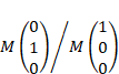

The harmonic terms, and , are developed from (those for are similar)

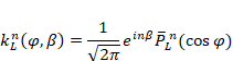
where the normalized associated Legendre functions, , are defined via a Fourier expansion as

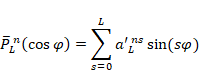
for n even and

for n odd. Each sum is only over either the even or odd values of s, respectively, because of the properties of the Fourier coefficients, . These Fourier coefficients are determined so that the definition

is satisfied. Terms of the form and are combined depending on the symmetry and the value of n along with appropriate normalization coefficients to give the harmonic terms and . For cubic crystal symmetry, the term is obtained directly from the Fourier expansion

using the coefficients, , as tabulated by Bunge (1982).

Note that this version of the general axis equation differs from that shown in Von Dreele (1997) in that the assignment of m and n are reversed.

The Rietveld refinement of texture then proceeds by constructing derivatives of the profile intensities with respect to the allowed harmonic coefficients, , and the three sample orientation angles, W_s, C_s, F_s, all of which can be adjustable parameters of the refinement. Once the refinement is complete, pole figures for any reflection may be constructed by use of the general axis equation, the refined values for and the sample orientation angles W_s, C_s, F_s.

The magnitude of the texture is evaluated from the texture index by

If the texture is random then J = 1, otherwise J > 1; for a single crystal J = ¥.

In GSAS-II the texture is defined in two ways to accommodate the two possible uses of this correction. In one, a suite of spherical harmonics coefficients is defined for the texture of a phase in the sample; this can have any of the possible sample symmetries and is the usual result desired for texture analysis. The other is the suite of spherical harmonics terms for cylindrical sample symmetry for each phase in each powder pattern (“histogram”) and is usually used to accommodate preferred orientation effects in a Rietveld refinement. The former description allows refinement of the sample orientation zeros, W_s, C_s, F_s, but the latter description does not (they are assumed to be zero and not refinable). The sample orientation angles, (W, C, F) are specified in the Sample Parameters table in the GSAS-II data tree structure and are applied for either description.

Some useful examples:

1) Bragg-Brentano laboratory powder diffractometer

The conventional arrangement of this experiment is to have a flat sample with incident and diffracted beams at equal angles (theta) on opposite sides of the sample. The sample is frequently spun about its normal to improve powder statistics and impose cylindrical symmetry on any preferred orientation (texture). Thus, the diffraction plane (source, diffraction vector & detector) contains the K-vector which is parallel to the diffraction vector and W, C, F = 0.

2) Debye-Scherrer diffractometer with point detector(s)

The usual arrangement here is to have a capillary sample perpendicular to the diffraction plane. The capillary may be spun about its cylinder axis for powder averaging and to impose cylindrical symmetry on the texture which is perpendicular to the diffraction plane. Thus, W, F = 0 and C =90.

3) Debye-Scherrer diffractometer with 2D area detector

The area detector is presumed to be directly behind the sample with the incident beam somewhere near the center of the detector. The detector axes are defined (for a synchrotron) with the X-axis toward the synchrotron ring and the Y-axis vertical “up”; one views the detector image as if looking from the x-ray source. The sample is assumed to be a capillary (which may be spun to impose cylindrical symmetry), although other sample shapes may be used, and is aligned with the cylinder axis horizontal. Integration of the image from a series of “caked” slices gives a set of powder patterns, each assigned an azimuthal angle where zero is along the X-axis. Thus, at azimuth=0 the diffraction plane is horizontal and contains the cylinder axis so W, C, F = 0.

In this tutorial we will use both of these descriptions to determine the texture of the two phases in a NiTi shape memory alloy sample with cylindrical symmetry (wire texture) as collected at APS on beam line 1ID-C (data kindly provided by Paul Paradise & Aaron Stebner of Colo. School of Mines) with the sample mounted so the cylinder axis was vertical. Thus, there are three ways within GSAS-II that can be used for this texture analysis all beginning with the same 2D area detector image. Each will be described in turn after the initial setup of the GSAS-II project, image input & integration.

Step 1. Image input & integration

If you have not done so already, start GSAS-II. Note that menu entries are listed in bold face below as Help/About GSAS-II, which lists first the name of the menu (here Help) and second the name of the entry in the menu (here About GSAS-II).

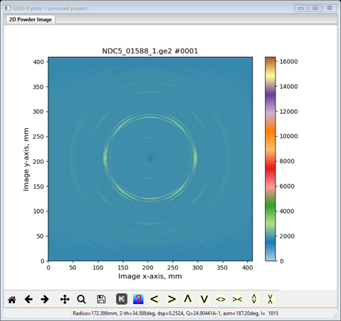
Use the Import/Image/from GE image file menu item to read the data file into the current GSAS-II project. A file selection dialog will be shown; its appearance will depend on your OS. Change the search directory to 2DTexture/data and then select the file NDC5_01588_1.ge2. An image will appear

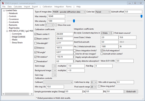
and the Image Controls data page will show

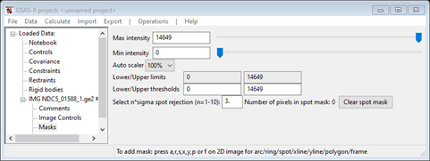
The detector was previously calibrated, and the coefficients are stored in a file found by doing Parms/Load Controls from the Image Controls menu. A file selection popup will appear showing NDC5.imctrl; select it and press Open. The Image Controls window will be repainted with the new values and the image will be redrawn.

The detail in the image can be enhanced by lowering the Max intensity (15000 is suitable) and shows that the diffraction rings show the effect of texture and that the image has a fairly high background. Placing the cursor in the corners or inside the inner ring shows a background >1700. This can be suppressed by adjusting the Flat Bkg (I chose 1700 for this). The image will now show the rings much more clearly.

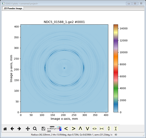
For texture analysis we will need to integrate the image into a number of slices sampling the changing ring intensity with azimuthal angle. Also note that the image seems to have mm symmetry so that the unique part of this intensity variation covers 0-90° of azimuth. In addition, the ring intensity variation is such that using 10° slices will capture it reasonably well. However, we want to include both 0° and 90° as slice centers. Thus, there will be 10 slices beginning at -5° and ending at 95°. Check the Show integration limits? box and uncheck the Do full integration? box, enter 10 in the No. azimuth bins, enter -5 in the Start azimuth box (it will change to 355) and enter 455 in the End azimuth box. In addition, recall that the sample was mounted vertically and thus is aligned with the defined laboratory I axis. Thus, the sample coordinate system needs to be rotated by 90° to match the sample axis with the K axis; this can be done by making the Sample goniometer axis Chi = 90. The plot will change with each entry and at the end should look like

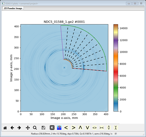
The Image Controls should be

It turns out that the image contains a number of “picked bits” (very high count “zingers”); these can be mostly eliminated by setting the upper threshold in Masks. Select Masks and the following should appear

Change the Upper threshold to 2500; the image will be redrawn reflecting this mask. By zooming in you may see isolated red pixels; these are excluded points. Make sure the diffraction rings do not have any excluded points. For example, with the level set to 2200 the plot shows

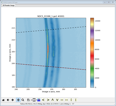
for one ring. This level is too low. Return to the Image Controls item in the data tree.

We are now ready to integrate the image; do Integration/Integrate from the Image Controls menu. When done the last powder pattern in the tree will be displayed

Step 2. Enter NiTi phases

This NiTi alloy consists of two phases, cubic B2 and monoclinic B19’. Their parameters are:
B2: P m 3 m, a=3.0240, Ni 0,0,0, Ti ½,½,½, U_iso=0.005 for both.
B19’: P 1 1 21/m, a=2.8853, b=4.6353, c=4.1368, γ=96.821, Ti 0.5787,0.2841,¼, Ni 0.9700,0.8209,¼, U_iso=0.005 for both.
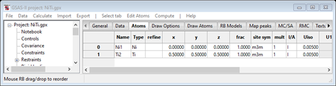
Use the Data/Add new phase to enter the B2 and B19’ phases; then for each enter the information given above on their respective General and Atoms tabs. Don’t forget the spaces between the axial fields for the space group symbols. On the Atoms tab begin by doing Edit Atoms/Append atom twice then fill in the Type and coordinates boxes. A double click of the Type entry will show a popup of the Periodic Table; select the element as appropriate. NB: GSAS-II happily takes “1/2” & “1/4” for coordinate values; these get converted to their decimal equivalent upon entry. 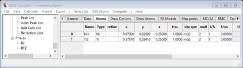Note the use of a nonstandard space group designation for B19’. When done the B2 Atoms table should look like

and the B19’ Atoms table should be

Next go to the Data tab for each phase; there will be a message indicating the lack of data for each. Do Edit Phase/Add powder histograms, do Set All on the popup selection window and press OK. The window for B2 will change to

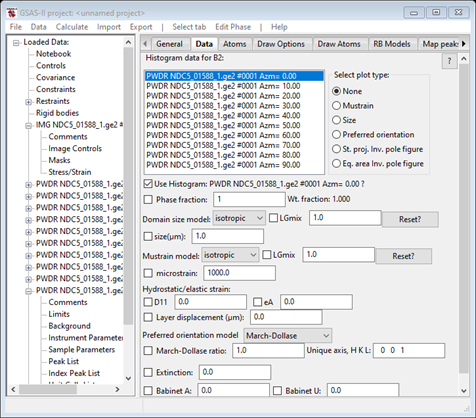
and that for B19’ will be

You should now save the project file (I used NiTi for a name); we will use this as a starting point for three different texture determinations. Do a File/Save project as… and give it a new name (I used NiTi-A); this will become the new project name for the next part of this tutorial.

Method A. Full refinement

Introduction

In this method we will do a full Rietveld refinement of the texture, profile parameters, peak position variables and crystal structure parameters. This is suitable in this case because of the relatively small number of histograms (10 in this case) needed for the texture determination; do recall that each phase in each histogram has a set of parameters (e.g. phase fraction, size, mustrain & hydrostatic strain) in addition to the ones for each histogram (e.g. background & scale factor). Consequently, the total number of parameters can build up very quickly in this method of analysis. The other two methods seek to reduce this problem by splitting the fitting into a sequential refinement (histogram by histogram) step followed by a texture fitting step.

Step 1. Initial refinement

In the initial refinement we need to vary the phase fraction for each phase/histogram and the background in each histogram. To start select any PWDR entry from the GSAS-II data tree and select Sample Parameters for it. Note that Goniometer chi is set to 90; that came from the same entry in the Image Controls during integration. Also, if you chose other than the 1^st PWDR data set, the Detector azimuth will be some nonzero value; that is also reflected in the name assigned to the histogram (e.g. PWDR NDC5_01588_1.ge2 Azm= 40.00). Uncheck the Histogram scale factor box and then do Command/Copy flags; select Set All and then press OK. That will clear the scale factor refinement flag for all histograms; we will be varying the phase fractions instead.

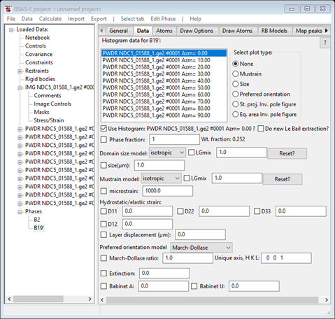
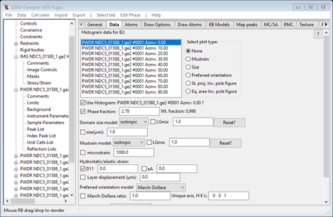
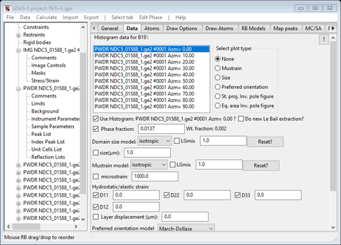
Next select the B2 phase and pick the Data tab; you will see

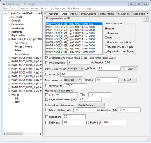
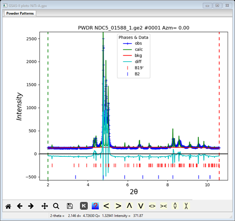
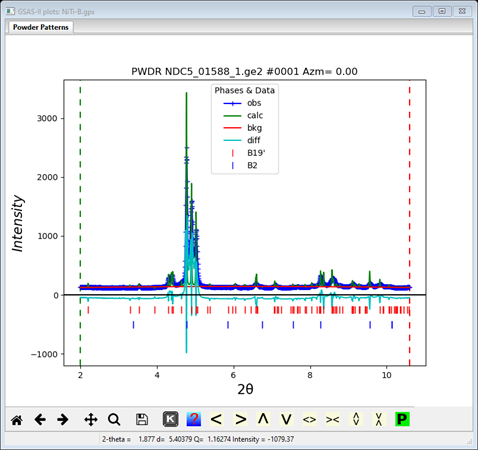
Select the Phase fraction box. Then do Edit Phase/Copy data, select Set All & press OK to copy these to the other histograms. Next select the B19’ phase and repeat this process. We are now ready for the first refinement; do Calculate/Refine from the main GSAS-II data tree window. A progress bar popup will appear and when done a Refinement results popup will show with Rw~33%. Press OK to load this result; GSAS-II will return you to the last window you were using and display (NB: pick the 1^st PWDR entry) the 1^st powder pattern showing you the fit

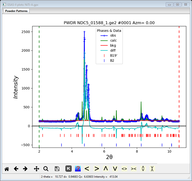
This is quite poor. You can survey the fit successively by 1^st selecting say the 1^st PWDR entry from the tree and then using the up/down arrow keys to step to the next one; the plot will redraw at each step (NB: at the same scale as the 1^st one selected) and the data window will show statistics of the fit. There is a substantial intensity discrepancy; this is due to the texture. It is also evident that some of the peaks are out of place relative to the reflection markers; this is due to macroscopic strain in the drawn wire. For the B2 phase select the Texture tab; it should look like

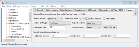
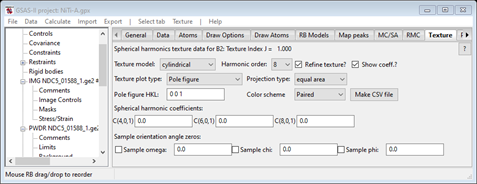
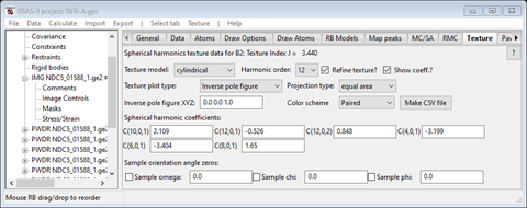
The texture model is cylindrical by default; that is what we want. Change the Harmonic order to 8 and check both Refine texture and Show coeff. The window should look like

Then go to the Data tab, select D11; the Data window should look like (any PWDR item will do)

Then do Edit Phase/Copy flags to have D11 refined for all PWDR data sets.

Next select the B19’ phase Texture tab. Then select 6 for the Harmonic order and check the two boxes as before.

Then go to the Data tab for the B19’ phase and check all 4 of the Dij boxes and do Edit Phase/Copy flags as before. The tab will look like

Now do Calculate/Refine from the main menu. The refinement will finish with Rw ~29%; the 1^st PWDR pattern looks like

The calculated peaks for both phases are too sharp. It is likely that this is a microstrain effect. Select Data for the B2 phase and select the microstrain box. Then do Edit Phase/Copy flags to set it for the other PWDR data sets. Do the same for the B19’ phase. Then do Calculate/Refine from the main menu. The fit will be substantially improved with Rw ~14%.

Step 2. Finish refinement and examine texture

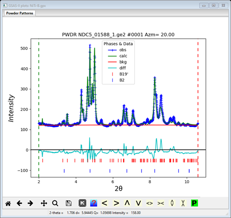
Looking at the individual PWDR data sets (e.g. the one for Azm=20.00)

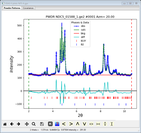
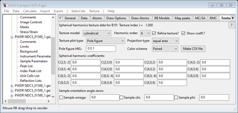
It is evident that there remain intensity differences due to texture. We can increase the harmonic order to more closely fit these, however one should do this carefully. Select the Texture tab for the B2 phase; the Texture tab will show

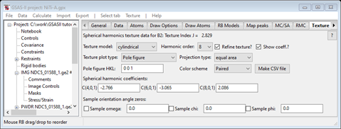
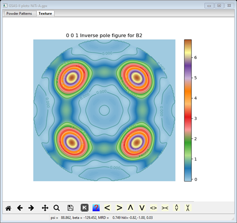
And a drawing of the 001 pole figure will be drawn. This is the very typical “bulls eye” for cylindrical texture; of much more use is an inverse pole figure. Select that from the Texture plot type; the plot will be redrawn

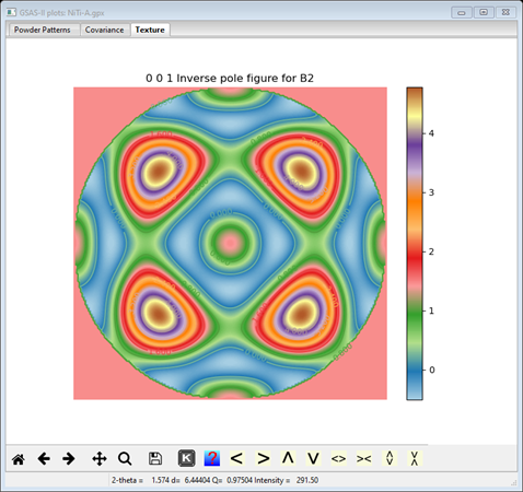
This shows the probability of reflection vectors coinciding with the sample wire axis; the high spots are the 111 family of reflections. We should try the next higher harmonic order (10).

Next go to the Texture tab for the B19’ phase. Again, a bullseye pole figure is drawn; change that to an Inverse pole figure.

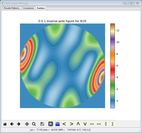
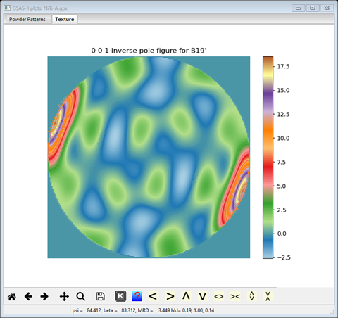
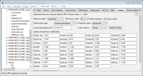
This phase is very strongly textured (the cursor shows 12-13 MRD at the peaks) along the -140 direction. Again, we want to increment the Harmonic order to the next higher level (8). Again, do Calculate/Refine from the main menu; the Rwp has dropped to ~10.4%. One can add the atom Uiso for the Ni and Ti atoms in the B2 phase and the coordinates and Uiso for the B19’ phase. The Rw drops a bit further to ~8.4%. Finally, we can increase the harmonic order again for the B19’ phase (it is very strongly textured!) to 10 and the B2 phase to 12; the final refinement converged to Rw ~7.9% and the B19’ inverse pole figure has peaks at ~18 MRD (Multiple of Random Distribution) and the B2 phase peaks are ~7MRD.

The B19’ coefficients

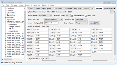
and inverse pole figure

The B2 coefficients

and inverse pole figure

This completes the tutorial on Method A for doing texture analysis. It is useful for a case like this one where there are very few data sets required for the texture analysis. However, for the case of lower sample symmetry one must have several dozen or even a few hundred histograms and then the suite of parameters can easily be > 1000 of which only a few dozen describe the texture. This leads to the next Methods for texture analysis in GSAS-II.

Method B. Sequential refinement & texture analysis from result

Introduction

This begins the texture analysis in much the same way as Method A except that all the initial refinements are done “sequentially”, that is refinements are done for the parameters associated with each powder pattern to convergence in a serial fashion. In this case where there are 10 PWDR data sets, there will be 10 refinements done in sequence. Parameters that span all the data (e.g. lattice parameters, atom parameters & texture) are not varied in this sequence refinement. The effect of texture is modeled as a Preferred Orientation correction to each histogram. To begin do File/Open project… for the NiTi.gpx file created in the first step and then do a File/Save project as… to save it as NiTi-B. This renames the project and it should have one IMG, 10 PWDR entries and two phases of NiTi (B2 and B19’).

Step 1. Initial refinement

This begins the same way as Method A so I’ll be brief. Do the following steps:

1) Select any PWDR entry, go to Sample Parameters and uncheck Histogram scale factor. Then copy the flags to the other PWDR entries.

2) Select the B2 phase Data tab and check the Phase fraction box and change the Preferred orientation model to Spherical harmonics. Then do Edit Phase/Copy data to copy both the flag and the model to the other PWDR entries.

3) Select the B19’ phase Data tab and check the Phase fraction box and change the Preferred orientation model to Spherical harmonics. Then do Edit Phase/Copy data to copy both the flag and the model to the other PWDR entries.

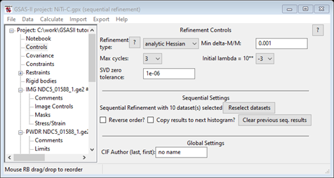
Now select Controls from the GSAS-II data tree

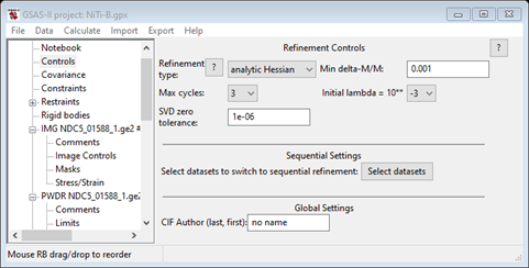
Press the Select datasets button for Sequential settings; a file selection popup will appear. Do Set All and press OK. The Controls page will be repainted indicating that 10 data sets are selected for sequential refinement.

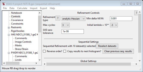
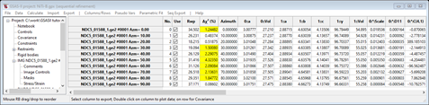
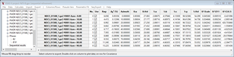
You have the choice of starting at the last one and for copying results from one to the next. We won’t do either here. Each refinement will use the other controls (e.g. Max cycles) as controls. We are now ready to do the 1^st sequential refinement. Do Calculate/Sequential refine from the main menu. A progress bar popup will appear showing residuals as it processes each of 10 data sets. After a few seconds the Refinement results popup will appear; press OK to accept them. The data window displays the Sequential refinement results as a table.

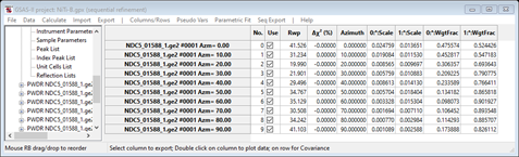
There is a row for each data set and columns for all refined parameters and some derived ones along with residual and convergence indicators. The residuals are not very good (we haven’t really refined much) but the Δχ² column shows that convergence was achieved (NB: poor convergence will be highlighted in yellow or red depending on how bad it is).

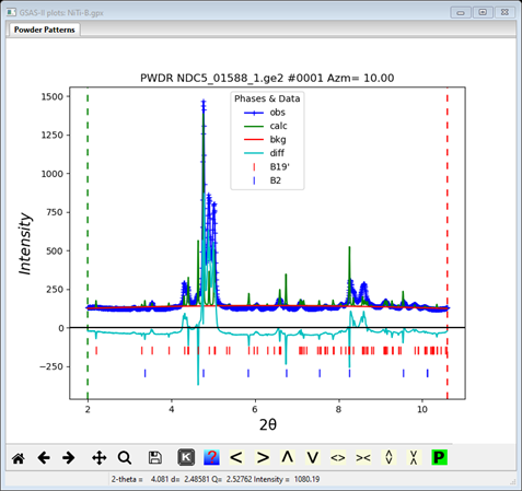
If you examine one of the PWDR entries, you’ll see that as at the same point in Method A much of the misfit is texture and perhaps peak position.

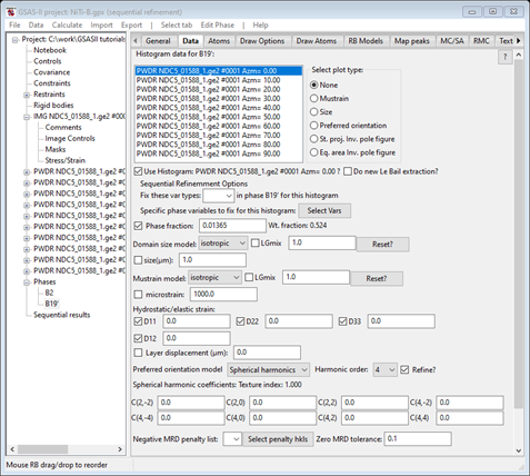
To set these parameters, select the Data tab for the B2 phase

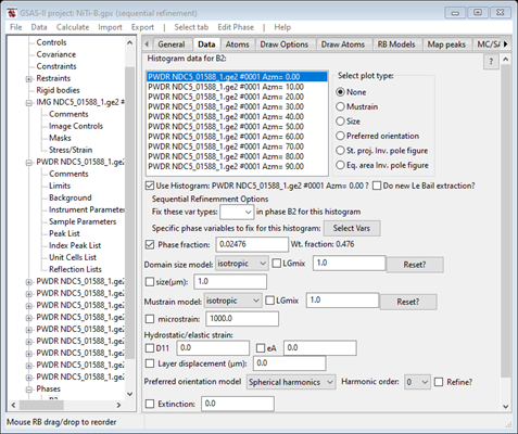
Check the D11 box under Hydrostatic/elastic strain, set the Harmonic order to 6 and check the Refine box for it (Preferred orientation). Then in two steps, first do Edit Phase/Copy flags and Set All for the file selection. Then do Edit Phase/Copy selected data; that will bring up a new popup

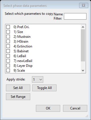
This allows you to select which parameters to copy data and flags. Select Pref. Ori. and press OK; the file selection is next. Do Set All and OK to do this copy. That copies the full spherical harmonics model to the other data sets. Select one to check if you’d like.

Next do the same thing for the B19’ phase; here there are 4 Dij parameters to check (do all of them) and use spherical harmonics order 4. When done that Data window will look like

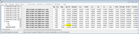
We are now ready for the next refinement; do Calculate/Sequential refine. After it completes the Sequential refinement results shows that the fit is better, but convergence wasn’t quite complete.

It is probably best to do another round of sequential refinement (I had to do two) to get convergence. A plot of one PWDR entry gives

As our experience in Method A, the calculated peaks are too sharp. We need to vary the mustrain parameters for both phases. Go to the Data tab for each phase, check the microstrain box and do Edit Phase/Copy flags for all the data sets. Then do another Calculate/Sequential refine. My Sequential refinement results showed great improvement but incomplete refinement

Repeating the sequential refinement (twice) gave convergence.

Examination of the PWDR data sets showed a fairly good fit but some discrepancies (especially for Azm=20.00)

Showing that perhaps the B19’ phase needs high order spherical harmonics. Select the Data tab for the B19’ phase and change the Harmonic order to 6. Then do Edit Phase/Copy selected data for Pref.Ori. to the other data sets. This (after few repeats) gives a further improvement in the fit

This fit is now sufficient for us to proceed to the next step and determine the texture of the two phases.

Step 2. Texture analysis

During the sequential refinements done in Step 1, we fitted the profiles allowing strain parameters (Dij) for peak position shifts and microstrain for peak shape. We modeled the intensity variation with a spherical harmonics preferred orientation correction. If you select any PWDR entry from the GSAS-II data tree and pick the Reflection List subentry (at the bottom) you can see the magnitude of this correction for each reflection in each phase.

For the B2 phase we see

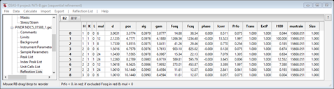
and for the B19’ phase we see

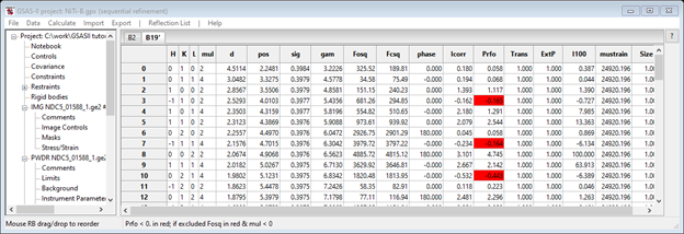
The preferred orientation correction is Prfo; notice a few entries in red. These are nonphysical correction values (physically, the correction can’t be negative) but by in large these are small. This next step uses these corrections as input data for a texture refinement. To start select the Texture tab for the B2 phase; you’ll see

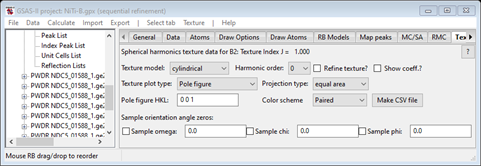
Since this sample has wire texture, we’ll use the default Texture model (cylindrical). Then set the Harmonic order to 12 (what we used earlier) and check the Refine and Show coeff boxes. The data window will be redrawn (and an orange blank plot will appear).

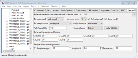
Do Texture/Refine texture from the menu; the window will be repainted, and a bullseye pole figure will appear. Change the Texture plot type to Inverse pole figure to get a more useful plot

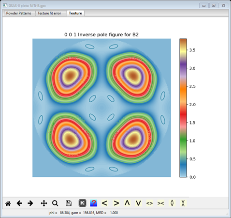
This is essentially the same as we obtained earlier in Method A (maybe not quite as strong here).

Now select the Texture tab for the B19’ phase and do the same; use Harmonic order 10 as we did earlier in Method A. After setting the two flags and doing Texture/Refine texture we get

and a bullseye pole figure; change that to Inverse pole figure to see the texture

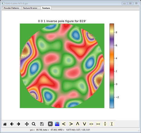
Again this is very similar to what we found in Method A but again not quite as strong (max MRD ~10 instead of ~18) and a bit choppier.

Now do a File/Save project from the main menu; this saves the final texture results done in Step 2 (you also will need it for Method C).

Method C. Sequential refinement & full texture refinement

Introduction

This uses the same approach as Method B except that after the sequential refinements are finished, we then fix almost all the parameters and then do a final texture refinement with all the data. Thus, this is a replacement for Step 2 in Method B. To begin do File/Open project… for the NiTi-B.gpx file created in Method B and then do a File/Save project as… to save it as NiTi-C. This renames the project and it should have one IMG, 10 PWDR entries and two phases of NiTi (B2 and B19’).

Step 1. Clearing unwanted variables from sequential refinement

Here we want to clear refinement flags for all parameters that need not be varied in a texture analysis refinement. The general rule is to not refine any parameter unless we expect it to affect the peak intensities. These are listed below:

1) Background: as the background was fit during the sequential refinement, we should fix it here. Select any PWDR entry and choose the Background subentry for it. Clear the Refine flags and the do Background/Copy flags selecting all data sets. This will clear all background refinement flags.

2) B2 phase: we do not want to refine either the microstrain, D₁₁, or preferred orientation coefficients. Select the B2 phase and its Data tab. Clear the microstrain, D₁₁ and Preferred orientation boxes. Also set the Harmonic order to zero (this will avoid a lot of nasty (but harmless) messages at the start of the refinement). Then do Edit Phase/Copy flags selecting all data to clear all the flags and an Edit Phase/Copy selected data for Pref.Ori to copy the zeroed out harmonic coefficients.

3) B19’: we do not want to refine either the microstrain, Dij, or preferred orientation coefficients. Select the B19’ phase and its Data tab. Clear the microstrain, four Dij and Preferred orientation boxes. Also set the Harmonic order to zero (this will avoid a lot of nasty (but harmless) messages at the start of the refinement). Then do Edit Phase/Copy flags selecting all data to clear all the flags and an Edit Phase/Copy selected data for Pref.Ori to copy the zeroed out harmonic coefficients.

Notice that we have allowed refinement of the Phase fractions; these may change during the texture refinement. Now select the Texture tab for the B2 phase (it may still have values from the Method B).

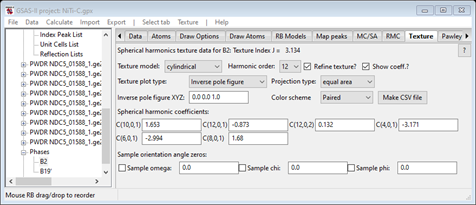
You can clear these by setting the Harmonic order to zero and then back to 12. Leave the Refine & Show boxes checked.

Then do the same for the B19’ phase. Select the B19’ phase and its Texture tab. Set the Harmonic order to zero and then back to 10. Leave the Refine and Show boxes checked. This completes the setup for the full texture refinement.

Step 2. Texture refinement

To clear the sequential refinement set up, select Controls from the main data tree.

Then do Reselect datasets, a popup window will appear

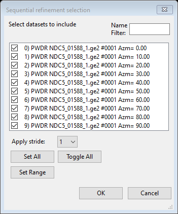
Do Toggle All to clear the check marks and press OK. The Controls will no longer show how many data sets are used in a sequential refinement.

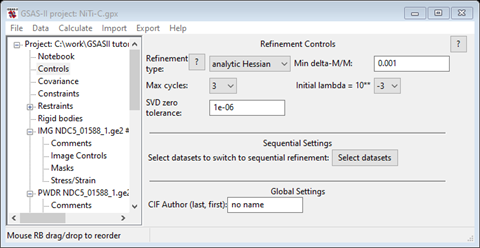
Do Calculate/Refine from the main menu; it will be a combined refinement on texture parameters.

A quick look at the console will show that there are 61 variables in this refinement. If yours shows more then you didn’t clear all the flags in Step 1. The Sequential results entry is deleted from the GSAS-II data tree. A progress bar will show giving the residuals during the refinement. When finished, select the B2 phase and its Texture tab; if the Texture plot type is still Inverse pole figure (from Method B) you should see

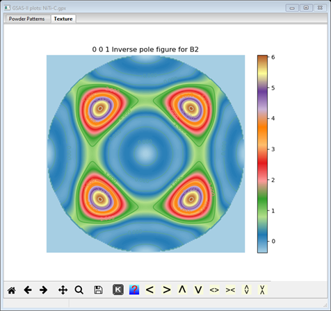
which is almost identical to that from Method A. The coefficients are seen in

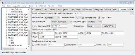
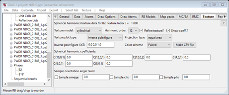
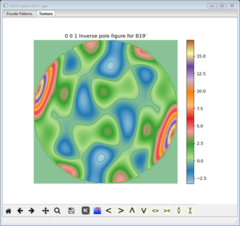
Now select the B19’ phase and its Texture tab; the inverse pole figure is

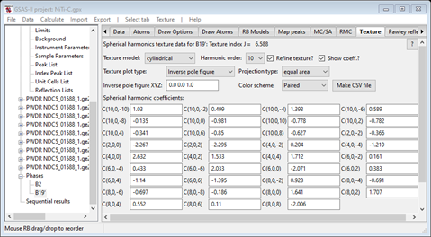
and also, almost identical to what was obtained in Method A; the coefficients are seen in

With this Method you can add parameters (atom coordinates & thermal motion parameters) that could not be refined in method B. It should be clear from this tutorial that in more complex textures where the data set may consist of slices obtained from a suite of 2D images collected as the sample is rotated, Method C will give a relatively fast determination of the texture without resorting to large matrix least-squares refinements.